Simulation Study: Evaluating the Hierarchical Bayesian Model

Overview

This vignette evaluates the performance of the hierarchical Bayesian model across a wide range of simulated scenarios. The study examines how well the model recovers the true population parameters ($\mu_0$, $\tau$, $\phi$) when individual observations are unavailable and only summary statistics are reported.

Three standard parametric families are considered — log-normal, Gamma, and Weibull — along with two extended families: Burr XII and Generalised Gamma (GG). Five summary-statistic types are evaluated:

summary_type	Fields reported
1	Median + range (min, max)
2	Median + IQR (Q1, Q3)
3	Mean + SD
4	Frequency table (rounded counts)
5	Mixed (multiple types across studies)

Note on Generalised Gamma identifiability. The GG distribution has three parameters ($\mu_0$, $\phi$, $\kappa$). In a hierarchical synthesis setting, certain combinations of summary-statistic types and sample sizes render the shape parameter $\kappa$ weakly identified. Scenarios flagged by the gg_heuristic rule are excluded from the summaries below; only scenarios where GG was judged estimable are retained.

Performance is assessed via:

• Credible-interval coverage — empirical 95% CI coverage for model parameters ($\mu_0$, $\tau$, $\phi$) and for two predictive quantiles (P50, P95); nominal target: 0.95.
• Median bias — median of (posterior median $-$ true value) across replicates for parameters and predictive quantiles; target: 0.
• Mean absolute error (MAE) — for model parameters.
• Integrated quadratic distance (IQD) and Weighted Interval Score (WIS) — measures of predictive distribution accuracy; lower is better.
• MCMC convergence rates — proportion of replicates with $\hat{R} < 1.05$.

Setup

library(ddsynth)
library(tidyverse)
#> ── Attaching core tidyverse packages ──────────────────────── tidyverse 2.0.0 ──
#> ✔ dplyr     1.2.1     ✔ readr     2.2.0
#> ✔ forcats   1.0.1     ✔ stringr   1.6.0
#> ✔ ggplot2   4.0.3     ✔ tibble    3.3.1
#> ✔ lubridate 1.9.5     ✔ tidyr     1.3.2
#> ✔ purrr     1.2.2     
#> ── Conflicts ────────────────────────────────────────── tidyverse_conflicts() ──
#> ✖ dplyr::filter() masks stats::filter()
#> ✖ dplyr::lag()    masks stats::lag()
#> ℹ Use the conflicted package (<http://conflicted.r-lib.org/>) to force all conflicts to become errors
library(ggsci)
library(here)        # used only for inst/extdata path resolution below
#> here() starts at /home/runner/work/ddsynth/ddsynth

Load Pre-computed Results

Running the full simulation study is computationally intensive. The results used here were generated by analysis/new_simulation_study.R and saved to disk. All scenario metadata (distribution family, summary type, sample sizes, true parameters) is embedded directly in the results file — no separate scenario library is needed.

# Resolve path: prefer the installed-package location; fall back to the
# vignettes/ source file which is tracked in git and available during
# pkgdown / R CMD build vignette builds.
rds_path <- system.file("extdata", "simulation_results_all.rds", package = "ddsynth")
if (!nzchar(rds_path)) {
  rds_path <- file.path(here(), "vignettes", "simulation_results_all.rds")
}
has_results <- file.exists(rds_path)
if (!has_results) {
  message("simulation_results_all.rds not found; skipping analysis chunks.")
} else {
  res_out <- readRDS(rds_path)
  cat(sprintf("Loaded %d simulation rows across %d unique scenarios.\n",
              nrow(res_out), length(unique(res_out$scenario_name))))
  cat(sprintf("Distribution families: %s\n",
              paste(sort(unique(res_out$dist_type)), collapse = ", ")))
  n_skipped <- sum(!is.na(res_out$skipped_reason))
  if (n_skipped > 0L)
    cat(sprintf("Note: %d rows excluded as non-identifiable (skipped_reason = '%s').\n",
                n_skipped, unique(na.omit(res_out$skipped_reason))))
}
#> Loaded 21900 simulation rows across 219 unique scenarios.
#> Distribution families: burr12, gamma, gengamma, lognormal, weibull
#> Note: 1060 rows excluded as non-identifiable (skipped_reason = 'gg_heuristic').

Summarise Results

create_results_summary() aggregates per-replicate outputs, restricting to converged, estimable runs. The resulting table contains, for each scenario:

• Coverage — empirical 95% CI coverage for $\mu_0$, $\tau$, $\phi$, and the predictive median (P50) and 95th percentile (P95).
• Median bias — median of (posterior median $-$ true value) for parameters and predictive quantiles.
• MAE — mean absolute error for parameters.
• IQD and WIS — mean predictive scoring rules across replicates.

summary_res <- create_results_summary(res_out)
cat(sprintf("Summary covers %d scenario-level rows.\n", nrow(summary_res)))
#> Summary covers 204 scenario-level rows.

Coverage of 95% Credible Intervals — Model Parameters

Each point represents one scenario. Points near the dashed red line (0.95) indicate well-calibrated uncertainty quantification. Points are coloured by the number of datasets and shaped by the within-study sample size.

create_coverage_plot(summary_res)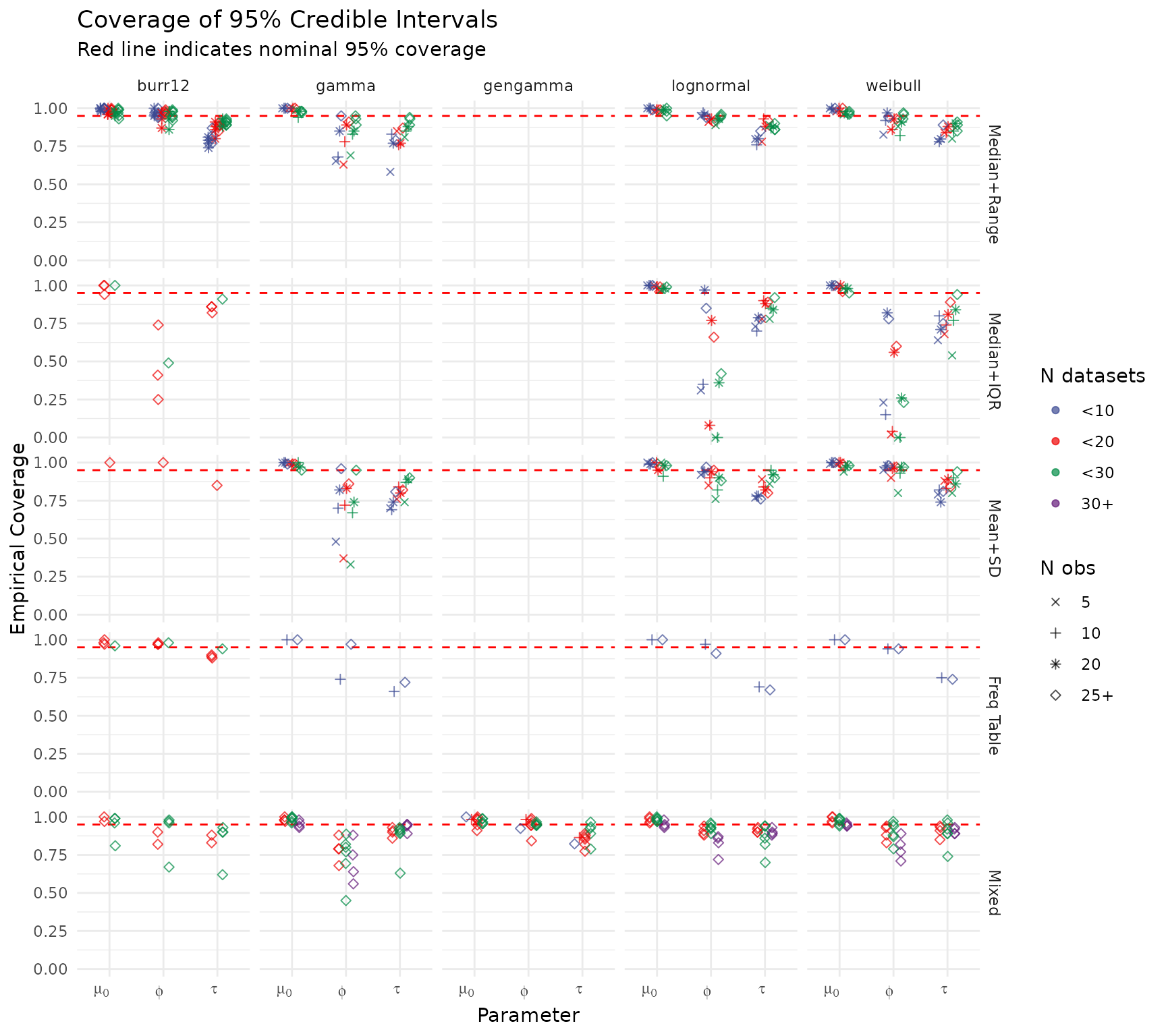

Median Bias — Model Parameters

The dashed red line at zero indicates unbiased estimation. Systematic departures from zero suggest that certain data configurations (e.g., very small $n$ or sparse summary types) introduce recoverable or persistent bias.

create_bias_plot(summary_res)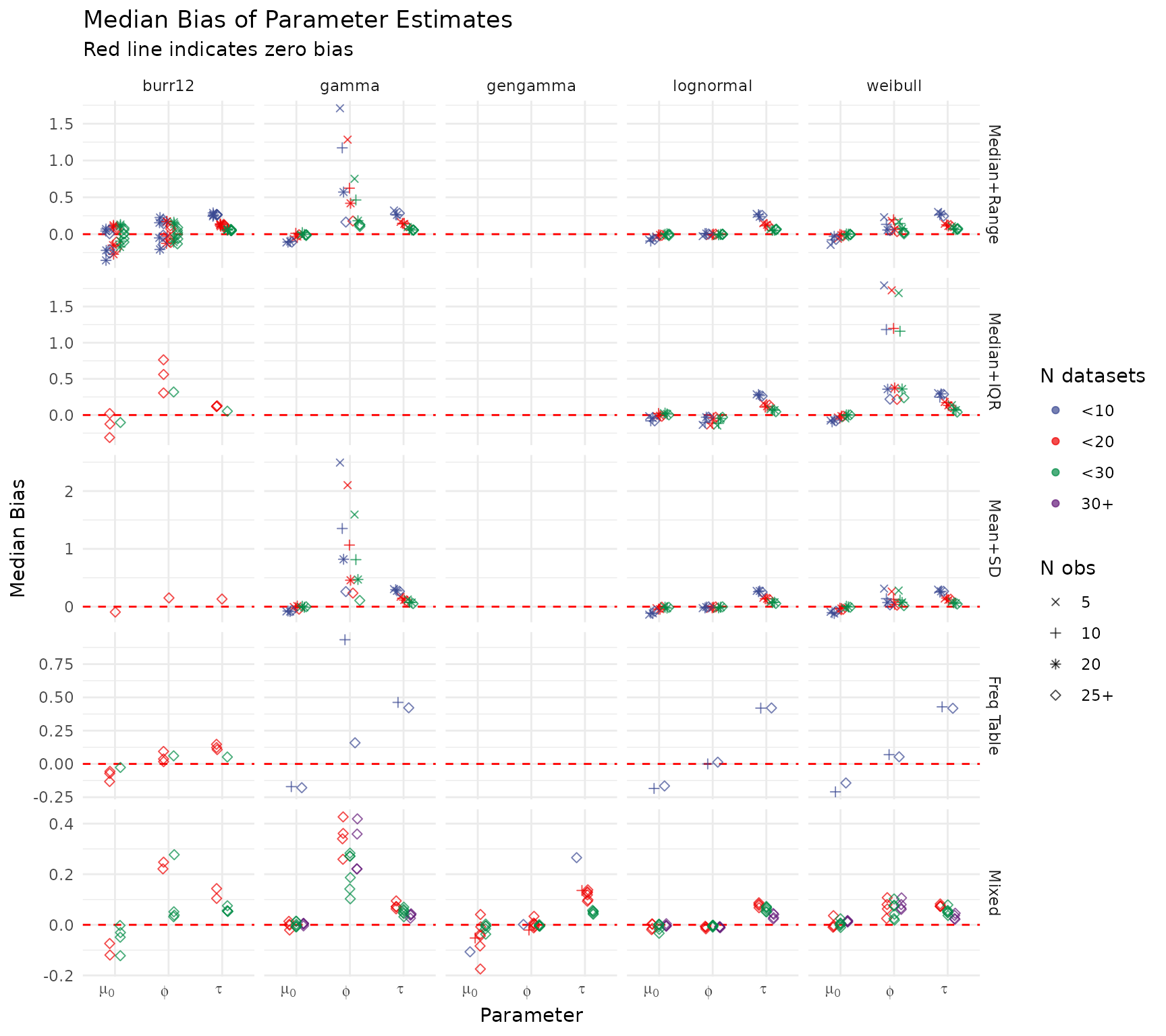

Mean Absolute Error — Model Parameters

MAE captures the magnitude of estimation error irrespective of direction. Smaller values across larger datasets and richer summary types confirm that pooling information across studies reduces estimation uncertainty.

create_mae_plot(summary_res)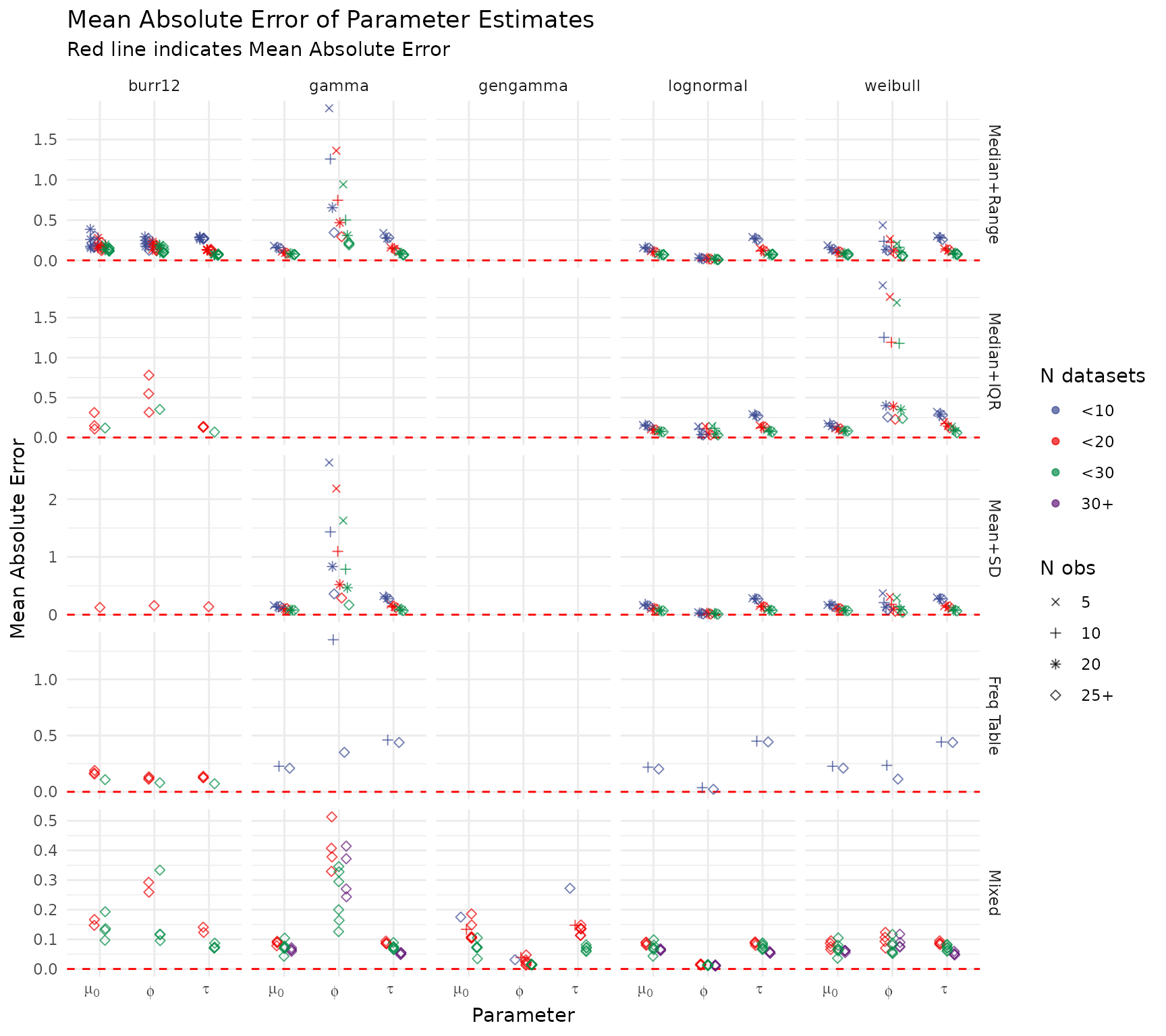

Coverage of 95% Credible Intervals — Predictive Median (P50)

Coverage for the posterior predictive median. Points near the dashed red line (0.95) indicate that the credible intervals reliably contain the true population median. Points are coloured by number of datasets and shaped by within-study sample size.

create_pred_median_coverage_plot(summary_res)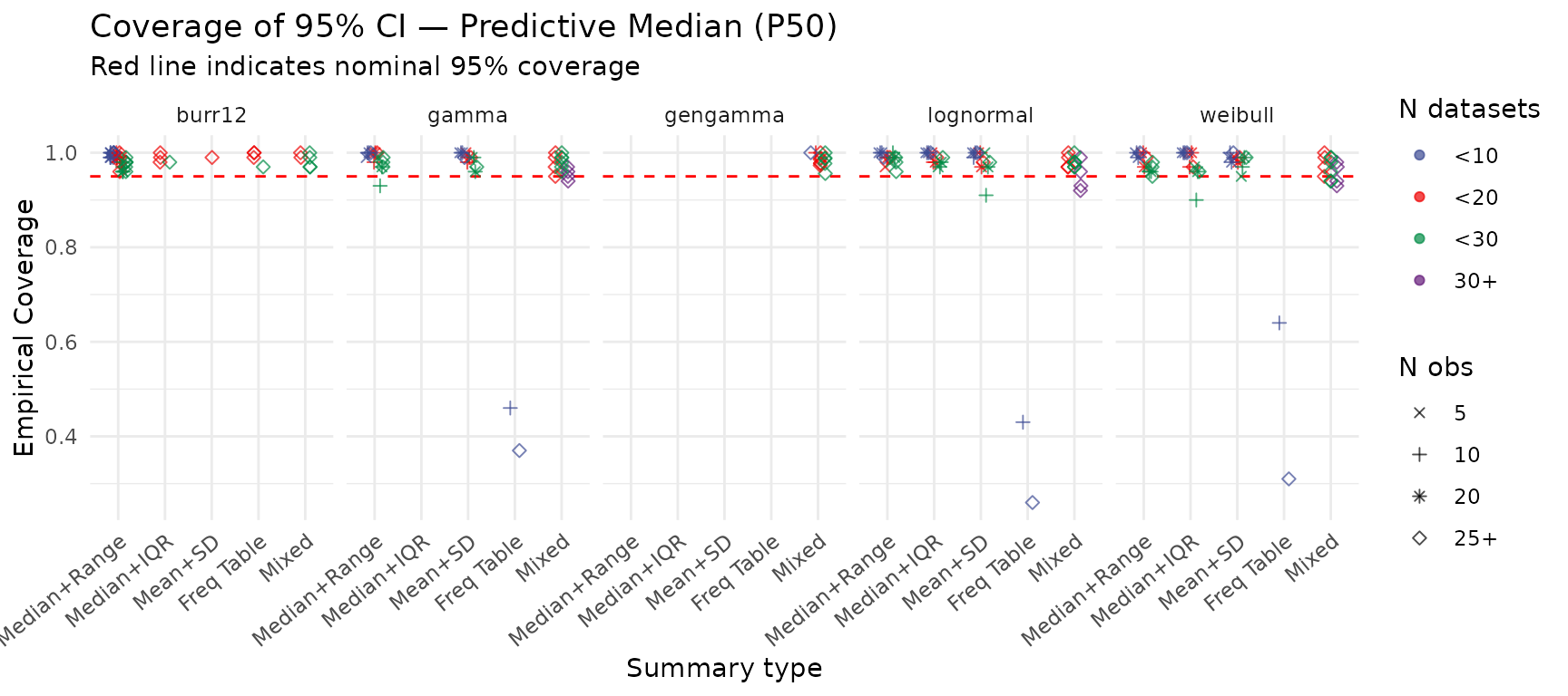

Coverage of 95% Credible Intervals — Predictive 95th Percentile (P95)

Coverage for the posterior predictive 95th percentile. Tail quantiles are typically harder to estimate and may show lower coverage in data-sparse scenarios.

create_pred_q95_coverage_plot(summary_res)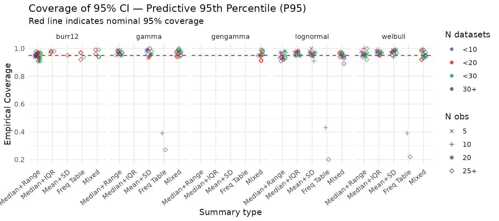

Median Bias — Predictive Median (P50)

Systematic over- or under-estimation of the predictive median across scenarios. Departures from zero can reflect inadequate pooling in sparse conditions.

create_pred_median_bias_plot(summary_res)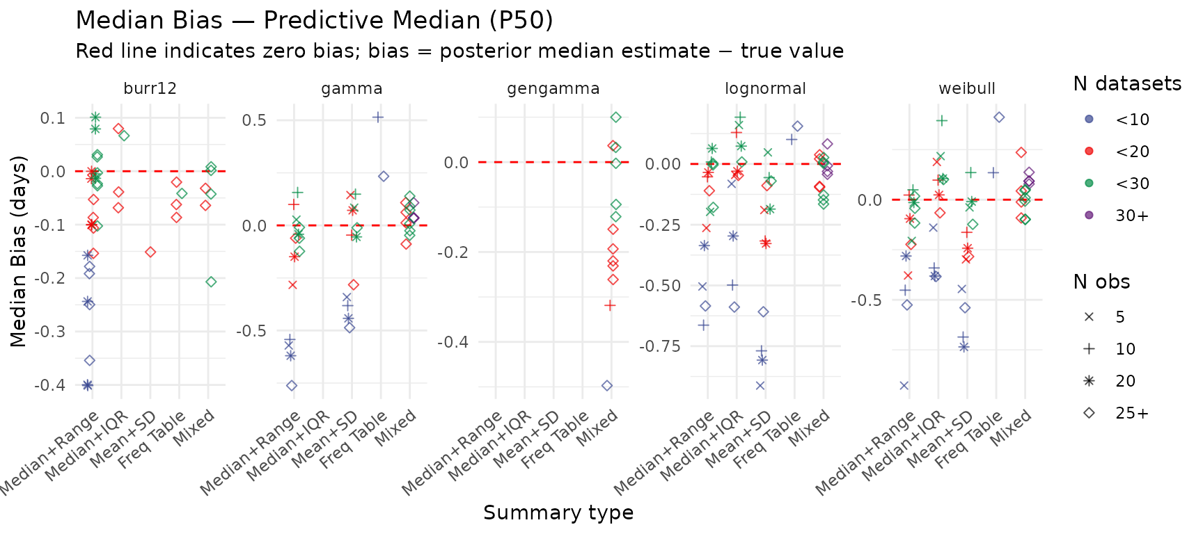

Median Bias — Predictive 95th Percentile (P95)

Bias in the posterior predictive 95th percentile. Persistent over-estimation of the tail is common when few datasets are available or the summary type provides limited information about the upper tail.

create_pred_q95_bias_plot(summary_res)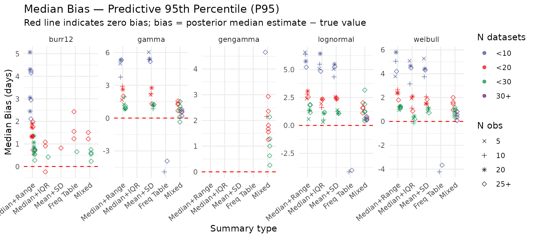

Integrated Quadratic Distance (IQD)

IQD measures the average squared discrepancy between the true and estimated predictive CDFs across the full support. Lower values indicate that the posterior predictive distribution closely matches the data-generating distribution.

create_iqd_plot(summary_res)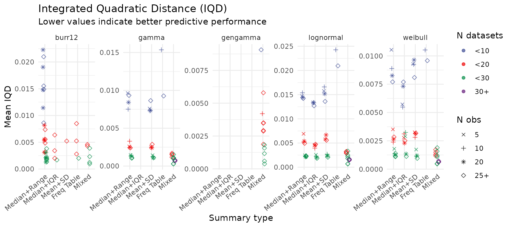

Weighted Interval Score (WIS)

WIS is a proper scoring rule that penalises both sharpness (narrow intervals) and miscoverage. Lower values indicate better overall predictive accuracy. Results here mirror the IQD analysis, providing a complementary view of predictive performance.

create_wis_plot(summary_res)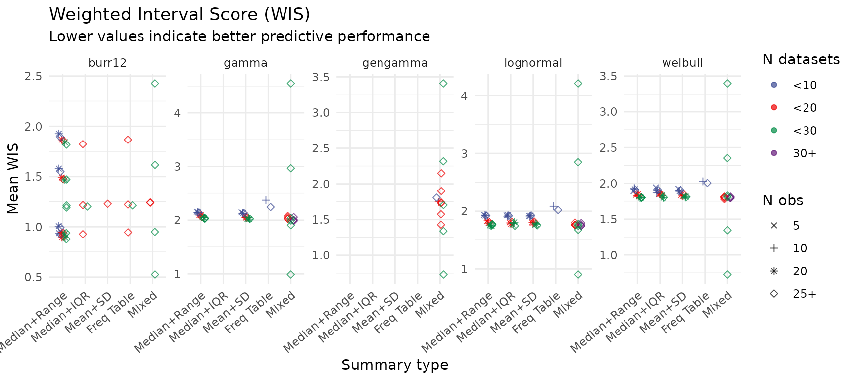

Summary Table

The table below aggregates all metrics across scenarios within each distribution-family × summary-type cell (averaging over number of datasets and within-study sample size). Coverage values are shown as percentages (nominal target: 95%). Predictive bias is the median signed error in days (target: 0). IQD and WIS are means over scenarios (lower = better).

library(kableExtra)
#> 
#> Attaching package: 'kableExtra'
#> The following object is masked from 'package:dplyr':
#> 
#>     group_rows

# Shared footnote text reused by both tables
.fn <- paste0(
  "Coverage: empirical proportion of replicates where the true value fell ",
  "inside the 95% posterior credible interval. ",
  "Predictive bias: median signed error (posterior median estimate \u2212 true value) across replicates. ",
  "IQD: integrated quadratic distance between true and estimated predictive CDFs. ",
  "WIS: weighted interval score. ",
  "Gen. Gamma scenarios with fewer than 10 identifiable replicates were excluded prior to aggregation."
)

# Helper: format a summarised data frame into a kable
.fmt <- function(dat) {
  dat %>%
    transmute(
      `mu0`   = sprintf("%.1f", cov_mu0  * 100),
      `tau`   = sprintf("%.1f", cov_tau  * 100),
      `phi`   = sprintf("%.1f", cov_phi  * 100),
      `P50`   = sprintf("%.1f", cov_p50  * 100),
      `P95`   = sprintf("%.1f", cov_p95  * 100),
      `P50 `  = sprintf("%+.2f", bias_p50),
      `P95 `  = sprintf("%+.2f", bias_p95),
      `IQD`   = sprintf("%.3f", iqd),
      `WIS`   = sprintf("%.2f", wis)
    )
}

# ── Table 1: distribution × summary type ─────────────────────────────────────
t1_dat <- summary_res %>%
  mutate(
    dist_label = factor(dist_type,
      levels = c("lognormal", "gamma", "weibull", "burr12", "gengamma"),
      labels = c("Log-normal", "Gamma", "Weibull", "Burr XII", "Gen. Gamma")),
    st_label = factor(summary_type, levels = 1:5,
      labels = c("Median+Range", "Median+IQR", "Mean+SD", "Freq Table", "Mixed"))
  ) %>%
  group_by(dist_label, st_label) %>%
  summarise(
    n_scen   = n(),
    cov_mu0  = mean(coverage_mu0,         na.rm = TRUE),
    cov_tau  = mean(coverage_tau,         na.rm = TRUE),
    cov_phi  = mean(coverage_phi,         na.rm = TRUE),
    cov_p50  = mean(coverage_pred_median, na.rm = TRUE),
    cov_p95  = mean(coverage_pred_q95,    na.rm = TRUE),
    bias_p50 = median(bias_pred_median,   na.rm = TRUE),
    bias_p95 = median(bias_pred_q95,      na.rm = TRUE),
    iqd      = mean(mean_iqd,             na.rm = TRUE),
    wis      = mean(mean_wis,             na.rm = TRUE),
    .groups  = "drop"
  ) %>%
  arrange(dist_label, st_label)

tbl1 <- bind_cols(
  t1_dat %>% transmute(
    Distribution  = as.character(dist_label),
    `Summary type` = as.character(st_label),
    `N` = n_scen
  ),
  .fmt(t1_dat)
)

kbl(tbl1,
    col.names = c("Distribution", "Summary type", "N",
                  "\u03bc\u2080", "\u03c4", "\u03c6",
                  "P50", "P95", "P50", "P95", "IQD", "WIS"),
    align   = c("l", "l", "r", "r", "r", "r", "r", "r", "r", "r", "r", "r"),
    caption = "Performance summary by distribution family and summary type") %>%
  kable_styling(bootstrap_options = c("striped", "condensed", "hover"),
                full_width = TRUE, font_size = 12) %>%
  add_header_above(c(" " = 3,
                     "Parameter coverage (%)" = 3,
                     "Predictive coverage (%)" = 2,
                     "Predictive bias (days)" = 2,
                     "Scoring rules" = 2)) %>%
  pack_rows(index = t1_dat %>% count(dist_label) %>% deframe()) %>%
  footnote(general = .fn, general_title = "Note: ")

Performance summary by distribution family and summary type

			Parameter coverage (%)			Predictive coverage (%)		Predictive bias (days)		Scoring rules
Distribution	Summary type	N	μ₀	τ	φ	P50	P95	P50	P95	IQD	WIS
Log-normal
Log-normal	Median+Range	14	98.8	85.6	93.5	98.8	94.2	-0.14	+2.48	0.007	1.82
Log-normal	Median+IQR	12	99.0	82.0	40.4	98.8	96.6	-0.04	+2.14	0.007	1.83
Log-normal	Mean+SD	12	98.1	83.9	89.8	98.3	96.0	-0.25	+2.47	0.008	1.83
Log-normal	Freq Table	2	100.0	68.0	94.0	34.5	31.5	+0.13	-4.09	0.023	2.05
Log-normal	Mixed	14	97.3	88.6	89.1	97.2	95.1	-0.02	+1.15	0.002	1.95
Gamma
Gamma	Median+Range	14	98.7	82.3	82.0	98.6	97.0	-0.09	+1.97	0.004	2.08
Gamma	Mean+SD	12	98.7	79.7	70.2	98.8	96.9	-0.05	+2.18	0.004	2.07
Gamma	Freq Table	2	100.0	69.0	85.5	41.5	33.0	+0.37	-4.42	0.012	2.31
Gamma	Mixed	14	97.5	89.3	74.2	97.3	96.9	+0.04	+0.72	0.001	2.19
Weibull
Weibull	Median+Range	14	98.3	84.9	90.8	98.1	96.1	-0.16	+2.09	0.004	1.84
Weibull	Median+IQR	12	98.5	75.9	30.8	97.8	97.1	+0.06	+1.52	0.004	1.86
Weibull	Mean+SD	12	98.7	84.2	94.6	98.5	97.2	-0.26	+1.67	0.004	1.85
Weibull	Freq Table	2	100.0	74.5	94.0	47.5	30.5	+0.27	-3.94	0.010	2.02
Weibull	Mixed	14	96.7	90.3	86.9	96.6	95.6	+0.04	+0.87	0.001	1.85
Burr XII
Burr XII	Median+Range	26	98.2	86.2	95.7	98.5	94.8	-0.09	+1.36	0.007	1.30
Burr XII	Median+IQR	4	98.5	86.2	47.2	98.8	97.8	+0.01	+0.66	0.003	1.29
Burr XII	Mean+SD	1	100.0	85.0	100.0	99.0	95.0	-0.15	+0.82	0.005	1.23
Burr XII	Freq Table	4	97.8	90.2	97.5	99.0	95.0	-0.05	+1.39	0.005	1.31
Burr XII	Mixed	6	95.3	84.3	88.3	98.7	96.0	-0.04	+0.67	0.003	1.33
Gen. Gamma
Gen. Gamma	Mixed	13	97.3	86.7	94.8	98.6	95.6	-0.15	+1.67	0.003	1.81
Note:
Coverage: empirical proportion of replicates where the true value fell inside the 95% posterior credible interval. Predictive bias: median signed error (posterior median estimate − true value) across replicates. IQD: integrated quadratic distance between true and estimated predictive CDFs. WIS: weighted interval score. Gen. Gamma scenarios with fewer than 10 identifiable replicates were excluded prior to aggregation.

Summary Table: By Data Availability

The table below pools results across distribution families and shows how performance varies with the number of datasets and within-study sample size, broken down by summary type. Rows are grouped by summary type.

t2_dat <- summary_res %>%
  mutate(
    st_label = factor(summary_type, levels = 1:5,
      labels = c("Median+Range", "Median+IQR", "Mean+SD", "Freq Table", "Mixed")),
    n_datasets_bucket = case_when(
      n_datasets < 10  ~ "<10",
      n_datasets < 20  ~ "<20",
      n_datasets < 30  ~ "<30",
      n_datasets >= 30 ~ "30+"
    ) %>% factor(levels = c("<10", "<20", "<30", "30+")),
    n_obs_bucket = case_when(
      n_obs == 5  ~ "5",
      n_obs == 10 ~ "10",
      n_obs == 20 ~ "20",
      n_obs > 25  ~ "25+"
    ) %>% factor(levels = c("5", "10", "20", "25+"))
  ) %>%
  group_by(st_label, n_datasets_bucket, n_obs_bucket) %>%
  summarise(
    n_scen   = n(),
    cov_mu0  = mean(coverage_mu0,         na.rm = TRUE),
    cov_tau  = mean(coverage_tau,         na.rm = TRUE),
    cov_phi  = mean(coverage_phi,         na.rm = TRUE),
    cov_p50  = mean(coverage_pred_median, na.rm = TRUE),
    cov_p95  = mean(coverage_pred_q95,    na.rm = TRUE),
    bias_p50 = median(bias_pred_median,   na.rm = TRUE),
    bias_p95 = median(bias_pred_q95,      na.rm = TRUE),
    iqd      = mean(mean_iqd,             na.rm = TRUE),
    wis      = mean(mean_wis,             na.rm = TRUE),
    .groups  = "drop"
  ) %>%
  arrange(st_label, n_datasets_bucket, n_obs_bucket)

tbl2 <- bind_cols(
  t2_dat %>% transmute(
    `Summary type` = as.character(st_label),
    `N datasets`   = as.character(n_datasets_bucket),
    `N obs`        = as.character(n_obs_bucket),
    `N`            = n_scen
  ),
  .fmt(t2_dat)
)

kbl(tbl2,
    col.names = c("Summary type", "N datasets", "N obs", "N",
                  "\u03bc\u2080", "\u03c4", "\u03c6",
                  "P50", "P95", "P50", "P95", "IQD", "WIS"),
    align   = c("l", "r", "r", "r", "r", "r", "r", "r", "r", "r", "r", "r", "r"),
    caption = "Performance summary by summary type, number of datasets, and within-study sample size (pooled over distribution families)") %>%
  kable_styling(bootstrap_options = c("striped", "condensed", "hover"),
                full_width = TRUE, font_size = 12) %>%
  add_header_above(c(" " = 4,
                     "Parameter coverage (%)" = 3,
                     "Predictive coverage (%)" = 2,
                     "Predictive bias (days)" = 2,
                     "Scoring rules" = 2)) %>%
  pack_rows(index = t2_dat %>% count(st_label) %>% deframe()) %>%
  footnote(general = .fn, general_title = "Note: ")

Performance summary by summary type, number of datasets, and within-study sample size (pooled over distribution families)

				Parameter coverage (%)			Predictive coverage (%)		Predictive bias (days)		Scoring rules
Summary type	N datasets	N obs	N	μ₀	τ	φ	P50	P95	P50	P95	IQD	WIS
Median+Range
Median+Range	<10	5	3	100.0	72.2	81.0	99.7	95.6	-0.57	+4.98	0.012	1.99
Median+Range	<10	10	3	100.0	79.0	85.7	100.0	96.3	-0.54	+5.05	0.011	2.00
Median+Range	<10	20	7	99.4	78.3	95.1	99.6	95.4	-0.34	+5.07	0.014	1.63
Median+Range	<10	25+	7	99.9	82.7	95.6	99.7	95.1	-0.35	+4.20	0.013	1.62
Median+Range	<20	5	3	98.7	82.3	80.0	99.0	97.3	-0.28	+2.40	0.004	1.92
Median+Range	<20	10	3	99.0	84.3	85.7	99.0	97.0	+0.02	+2.81	0.004	1.92
Median+Range	<20	20	7	98.3	85.4	92.7	99.0	95.4	-0.09	+1.89	0.005	1.56
Median+Range	<20	25+	7	99.1	88.4	95.0	98.7	95.0	-0.11	+1.80	0.004	1.55
Median+Range	<30	5	3	97.7	83.3	82.0	98.0	96.3	-0.20	+0.95	0.002	1.88
Median+Range	<30	10	3	97.0	85.7	85.7	96.3	93.7	+0.05	+1.35	0.002	1.87
Median+Range	<30	20	7	97.3	89.6	92.0	97.0	94.3	-0.00	+1.07	0.002	1.53
Median+Range	<30	25+	15	97.3	89.9	94.9	97.5	95.5	-0.02	+0.94	0.002	1.62
Median+IQR
Median+IQR	<10	5	2	100.0	68.5	27.0	100.0	97.5	-0.11	+5.08	0.010	1.94
Median+IQR	<10	10	2	100.0	75.0	25.0	100.0	98.5	-0.42	+4.32	0.009	1.89
Median+IQR	<10	20	2	100.0	74.9	89.5	100.0	96.0	-0.34	+5.54	0.010	1.92
Median+IQR	<10	25+	2	100.0	76.5	81.5	100.0	95.5	-0.49	+4.67	0.010	1.91
Median+IQR	<20	5	2	99.5	73.0	5.0	100.0	97.5	+0.07	+1.94	0.004	1.83
Median+IQR	<20	10	2	98.5	82.0	6.0	97.5	98.0	+0.11	+1.36	0.004	1.83
Median+IQR	<20	20	2	99.0	84.5	66.5	99.0	96.5	-0.00	+2.22	0.003	1.82
Median+IQR	<20	25+	5	97.8	86.4	53.2	98.6	97.2	-0.05	+0.91	0.004	1.52
Median+IQR	<30	5	2	97.5	66.0	0.0	97.0	98.0	+0.19	+0.28	0.003	1.80
Median+IQR	<30	10	2	98.0	81.0	0.0	93.5	96.0	+0.29	+0.18	0.003	1.81
Median+IQR	<30	20	2	98.0	84.0	31.0	97.0	96.0	+0.09	+0.76	0.002	1.80
Median+IQR	<30	25+	3	98.0	92.3	38.0	97.7	96.7	+0.07	+0.42	0.002	1.58
Mean+SD
Mean+SD	<10	5	3	99.7	75.3	78.3	99.7	97.7	-0.45	+5.27	0.011	2.00
Mean+SD	<10	10	3	99.7	76.3	87.0	99.7	97.7	-0.69	+4.34	0.011	1.98
Mean+SD	<10	20	3	99.7	75.3	91.3	99.3	97.7	-0.74	+5.40	0.011	1.98
Mean+SD	<10	25+	3	99.7	79.3	97.0	99.7	95.3	-0.54	+5.17	0.010	1.99
Mean+SD	<20	5	3	99.7	84.3	70.7	99.7	97.3	-0.19	+2.15	0.004	1.91
Mean+SD	<20	10	3	99.3	83.7	86.0	99.0	96.7	-0.16	+2.21	0.004	1.90
Mean+SD	<20	20	3	98.0	83.7	91.3	98.0	95.7	-0.24	+2.35	0.004	1.89
Mean+SD	<20	25+	4	98.8	82.8	94.5	98.8	97.2	-0.22	+1.57	0.004	1.74
Mean+SD	<30	5	3	97.3	80.0	63.0	98.0	95.7	+0.05	+1.28	0.002	1.87
Mean+SD	<30	10	3	96.0	90.7	80.7	95.7	94.3	+0.14	+1.18	0.002	1.88
Mean+SD	<30	20	3	97.7	89.0	87.0	97.3	97.3	-0.05	+1.08	0.002	1.87
Mean+SD	<30	25+	3	97.0	91.3	93.3	98.0	97.3	-0.07	+1.08	0.001	1.86
Freq Table
Freq Table	<10	10	3	100.0	70.0	88.3	51.0	40.3	+0.13	-4.22	0.017	2.16
Freq Table	<10	25+	3	100.0	71.0	94.0	31.3	23.0	+0.23	-3.93	0.013	2.09
Freq Table	<20	25+	3	98.3	89.0	97.3	99.7	95.3	-0.06	+1.55	0.006	1.34
Freq Table	<30	25+	1	96.0	94.0	98.0	97.0	94.0	-0.04	+0.65	0.002	1.21
Mixed
Mixed	<10	25+	1	100.0	82.3	92.4	100.0	94.9	-0.50	+4.65	0.009	1.81
Mixed	<20	10	1	98.3	86.4	98.3	100.0	94.9	-0.32	+2.15	0.004	1.75
Mixed	<20	25+	20	97.8	88.4	88.6	98.2	95.6	-0.05	+1.55	0.003	1.77
Mixed	<30	25+	27	97.2	87.3	87.9	97.8	96.5	+0.00	+0.74	0.001	2.00
Mixed	30+	25+	12	95.0	91.3	77.5	95.3	94.8	+0.06	+0.56	0.001	1.86
Note:
Coverage: empirical proportion of replicates where the true value fell inside the 95% posterior credible interval. Predictive bias: median signed error (posterior median estimate − true value) across replicates. IQD: integrated quadratic distance between true and estimated predictive CDFs. WIS: weighted interval score. Gen. Gamma scenarios with fewer than 10 identifiable replicates were excluded prior to aggregation.

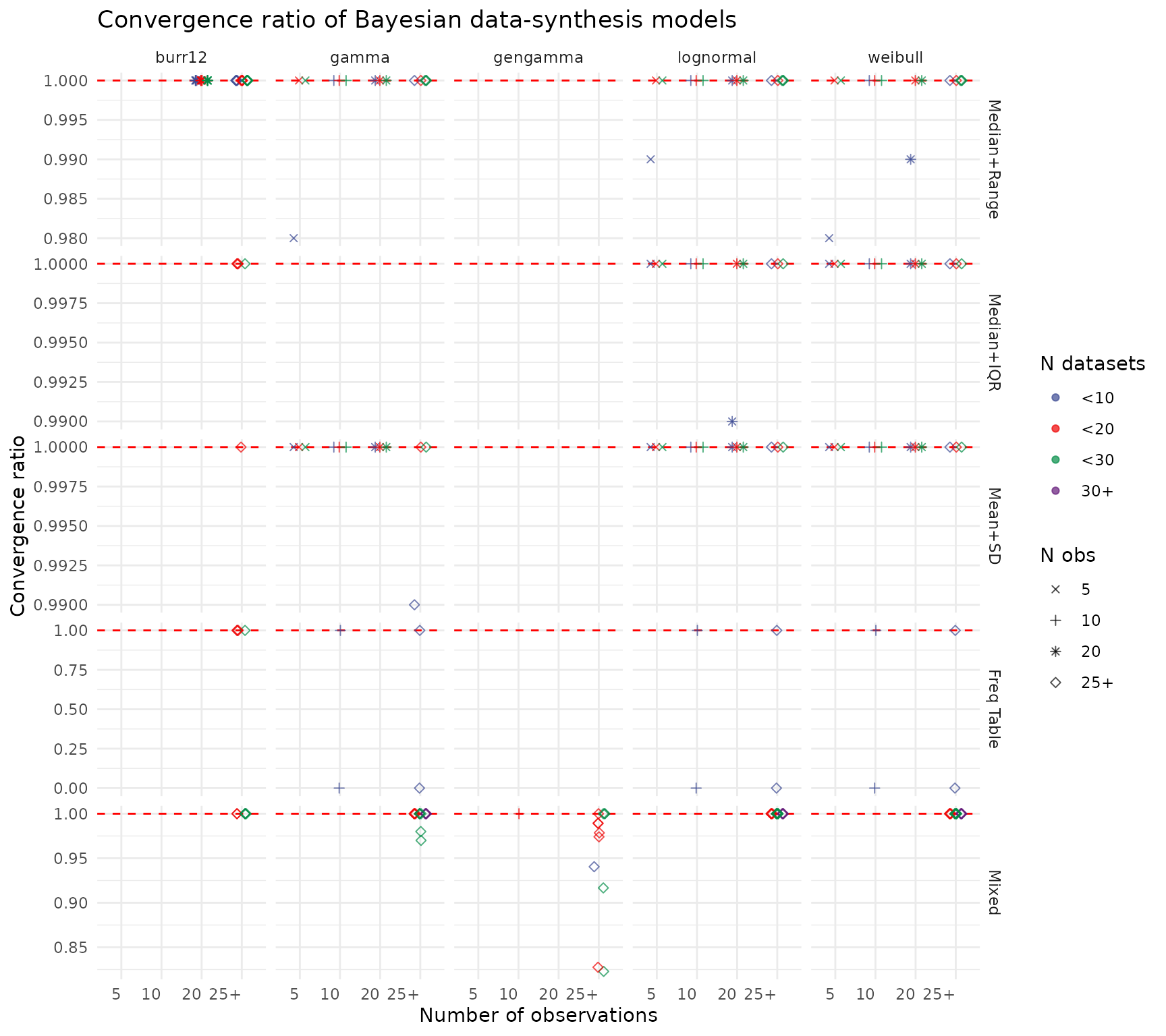
MCMC Convergence Rates

The convergence plot shows the proportion of simulation replicates where all chains reached $\hat{R} < 1.05$ and the effective sample size was adequate. Values at the dashed red line (1.0) indicate perfect convergence across all replicates. Lower rates in sparse conditions (few datasets, small $n$) highlight where the model may require more informative priors or additional iterations. Scenarios deemed non-identifiable (e.g. certain GG configurations) are excluded.

create_convergence_plot(res_out)